 by
by After working on binary classification in the kaggle competition with data from the Titanic , how about tackling another facet of machine learning? Multiple classification (Multi-class) through the recognition of figures / digit MNSIT (Modified National Institute of Standards and Technology database) is indeed a must in the initiation to Machine Learning. So let’s get carried away in this new Kaggle competition
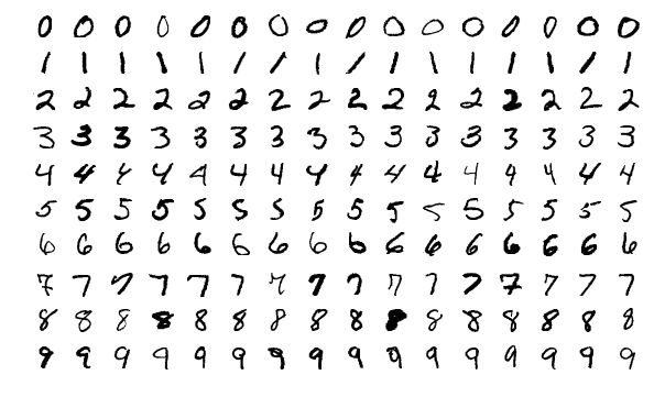
NB: The MNIST database for Modified or Mixed National Institute of Standards and Technology , is a database of handwritten numbers. The MNIST base has become a standard test. It brings together 60,000 training images and 10,000 test images, taken from an earlier database, simply called NIST 1 . These are black and white images, normalized centered 28 pixels per side. (Source: Wikipedia )
Index
Retrieve and read the dataset
To do this first register in the Kaggle competition , then retrieve the data in the data tab .
Here is the structure of the training and test files:
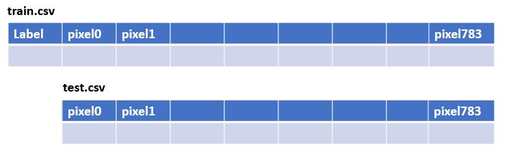
As usual of course the labels (label) are not present in the test data set… where would be the stake if not?
We have to process images. However, these images are bitmaps, that is to say they are represented via matrices of pixels. Each point / pixel is therefore an entry in the matrix. The value in the matrix defining the intensity of the point (gray level) of the image:
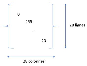
The only catch is that the data we recover is not exactly in this matrix format. in fact each image is flattened on a single line. We will therefore have to retrieve the entire row (without the label of course) and resize the row to a 28 × 28 matrix. Luckily the reshape () function comes to your rescue, but we’ll see that in the next chapter.
This step is not necessary if you do not wish to retouch or rework the images. You could quite simply run a machine learning algorithm directly on the matrix data online:
import pandas as pd
from sklearn.linear_model import SGDClassifier
pd.options.display.max_columns = None

TRAIN = pd.read_csv("./data/train.csv", delimiter=',') #, skiprows=1)
TEST = pd.read_csv("./data/test.csv", delimiter=',') #, skiprows=1)
X_TRAIN = TRAIN.copy()
X_TEST = TEST.copy()
y = TRAIN.label
del X_TRAIN["label"]

sgd = SGDClassifier(random_state=42)
sgd.fit(X_TRAIN, y)
print ("Score Train -->", round(sgd.score(X_TRAIN, y) *100,2), " %")
Score Train --> 85.88 %Without any adjustments and in a few lines you will have an honorable score of 85% (if you submit it as is to kaggle you will get 84% which is consistent). But of course we can do better, much better.
View images
The following portion of code retrieves a row from the dataset. The row is converted to a 28 × 28 matrix via the reshape () function and and visualized via matplotlib .
# returns the image in digit (28x28)
def getImageMatriceDigit(dataset, rowIndex):
    return dataset.iloc[rowIndex, 0:].values.reshape(28,28)
# returns the image matrix in one row
def getImageLineDigit(dataset, rowIndex):
    return dataset.iloc[rowIndex, 0:]

imgDigitMatrice = getImageMatriceDigit(X_TRAIN, 3)
imgDigit = getImageLineDigit(X_TRAIN, 3)
plt.imshow(imgDigitMatrice, cmap=matplotlib.cm.binary, interpolation="nearest")
plt.axis("off")
plt.show()
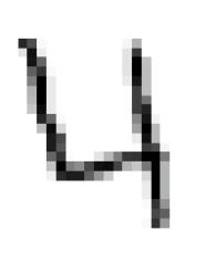
The result is then displayed:
Multi-class classification
In the Titanic project , we were in a binary classification type machine learning project. Indeed we had to determine whether the passengers were either survivors or dead. 2 possibilities only, hence the term binary classification. The multi-class classification extends this principle of classification to several labeling classes. This is exactly the case here because we have to classify the digits on the different possibilities [0..9].
In terms of Machine Learning algorithms, we therefore have two ways of handling this type of problem:
- Using binary classification algorithms. In this case it will be necessary to apply these algorithms several times by “binarizing” the labels. For example by applying an algorithm which will recognize the 1s, then the 2s, etc. This is what we call a strategy alone against everything (One versus All). Another method will consist of comparing the pairs / tuples to each other (One versus One)
- Using Multi-class algorithms. The scikit-learn library offers a good number of them:
- SVC (Support Vector Machine)
- Random Forest
- SGD (Stochastic Gradient Descent)
- K near neighbors (KNeighborsClassifier)
- etc.
Results analysis
In a previous chapter we started training on data with a Stochastic Gradient Descent (SGD) algorithm. We saw in another article how to analyze the results of a binary classification, but what about a multi-class classification?
Well, we’re just going to use the same analysis tools as the binary classification, but of course a little different.
The most practical tool in my opinion remains the confusion matrix . The difference here is we’ll read it differently.
sgd = SGDClassifier(random_state=42)
cross_val_score (sgd, X_TRAIN, y, cv=5, scoring="accuracy")
y_pred = cross_val_predict(sgd, X_TRAIN, y, cv=5)
mc = confusion_matrix(y, y_pred)
print(mc)
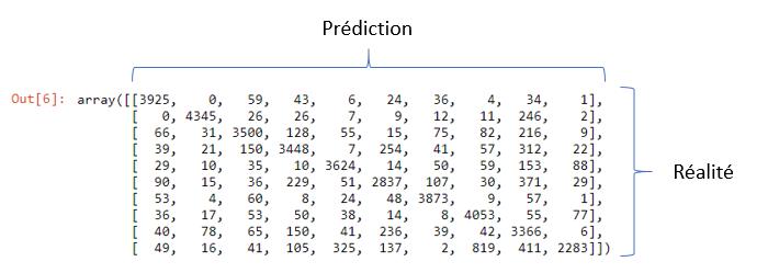
Here is the result :
The latter is very practical and allows you to compare by class (here I remind you [0..9]) the number of erroneous values between the prediction and the value actually observed. As a corollary, a confusion matrix being diagonal means a score of 100%! we will therefore only be interested in the values which are outside the diagonals, because they are those which point to the prediction errors.
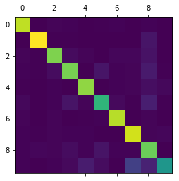
A visualization in the form of a heat map is also very useful. A simple call to matplotlib via the matshow () method and voila:
plt.matshow(mc)
First conclusions
In this first article we haven’t really done much yet. Reading the data and launching a first algorithm in order to get a first overview is essential and appears as the first step in order to get an idea of what we are going to implement subsequently to achieve our objective.
In a second article, we will see how to best use this dataset. For example, we could rework the information (for example by extending the dataset) or scale the raster data. And above all, finally, we will test and optimize our machine learning algorithms.